Solvers
This document’s purpose is to help navigate important and relevant information regarding how solvers in CST work, without reading 100+ page tutorials that can be somewhat difficult to navigate.
First, I summarize the purpose and usage of solvers in a general sense. Then, I talk about each specific kind of solver, explaining the methods the solver uses and when to use it. Finally, I help with navigating the solver windows by pointing out what each button and drop-down is intended for.
Solvers (Generally)
In general, the solvers that we are going to use are the Time Domain solvers and the Frequency Domain solver, and the others are for extremely specific situations. So I would emphasize understanding these solvers over the others for the sake of time.
Overview of Each Solver
CST typically will default to the solver it thinks is suitable, however ultimately the user must select the needed solver. Selecting the appropriate solver depends on the user’s knowledge, so I give the following information as a resource to aid in this. I describe each solver’s methods, usage and pros/cons.
Time Domain Solvers
There are two time domain solvers in CST, and each use hexahedral meshing. The two types are called the Transient solver and the TLM solver. They differ in the technique used, which I will go into below. When you go into Simulation: Solver => Setup Solver => Time Domain Solver, you have two meshing choices, Hexahedral and TLM Hexahedral. This is how you choose among the two kinds of solvers, where Hexahedral corresponds to the Transient solver and TLM Hexahedral to the TLM solver. However, for most applications the transient solver is preferable. For excitation signals, a Gaussian is used in the time domain.
Transient Solver
This solver is based on the Finite Integration Technique (FIT). It applies numerical methods like the Perfect Boundary Approximation (PBA) and the Thin Sheet Technique (TST). These techniques allow for robust meshing in return for efficient memory usage. The user can set up S-parameter symmetries or reciprocity, or AR-filtering to speed up the computation process. The solver stops when the energy inside the device is sufficiently close to zero.
This solver also uses an automatic mesh refinement. There are two ways that the solver will do the mesh refinement. The first one can be used anytime. The solver identifies the parts that are critical to electromagnetic behavior, and then refines the mesh in those regions accordingly. However, since these problems are complicated, a more accurate method will be the second choice. The mesh refinement is done based on results of a previous run.
This solver cannot handle periodic structures that have a nonzero phase shift, use the frequency domain solver instead.
TLM Solver
TLM stands for Transmission-Line Method, which is this solver’s technique. It is very similar to the Transient solver, except the TLM solver trades the ability to use certain materials with the ability to model extremely compact models. The exact applications will be discussed in the next section.
The biggest difference that the user needs to know when using TLM is the meshing. The TLM solver needs finer meshing than the Transient solver so that it can accurately portray the geometry. In order to reduce the total number of calculations, the solver will tighten the mesh cells closer to the geometry, clumping them together as it moves away. Also PBA is off in this solver (though it can be turned on).
The TLM solver uses a different excitation signal as well (though the signal can be changed if needed, but only after the initial calculation on the default setting which the following paragraph describes). The supported excitation types are discrete ports, plane waves, and field sources. Most waveguide ports are supported as well, but all waveguide ports MUST be excited. For the excitation signal, the solver applies an impulse excitation at the maximum model frequency and has a uniform magnitude across the frequency range of interest.
This solver is good for thin panels, coated metals, and shielded cables.
Frequency Domain Solver
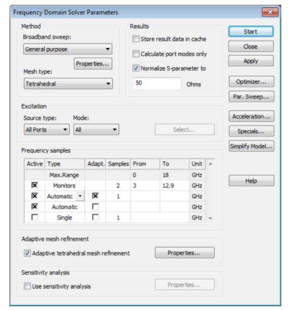
The Frequency Domain solver (FDS) differs from the Time Domain solvers in a way that can be derived from its name. It does more frequency samples, doing a complete simulation going from each frequency point to the next until the steps stop producing significantly different results. The frequencies in which the solver runs can be chosen or set to intervals (or both).
The FDS also uses a mesh refinement technique that differs from the one that the transient solver uses. FDS by default uses tetrahedral mesh, while the transient solver uses hexahedral. This is a good thing because it provides another independent method to verify results. And FDS only does the refinement for one frequency, which is chosen by the user. Usually the best point to chose is the one with the highest frequency within the range you are computing. Filters, however, should use a frequency within its pass band. The solver the refines the mesh best for that frequency, and then uses it for the rest of the calculations. However, it is possible to refine the mesh for multiple frequencies, but this makes the computation slower. If mesh refinement is wanted for multiple frequencies in steps, the user can set the convergence criterion, where the refinement stops after there is little significant change between steps.
This solver cannot handle nonlinear materials, so time domain solvers must be used. For large structures with many mesh cells, the frequency domain solver becomes very memory-intensive. If the mesh cells are in the order of several million, select either the time domain solvers or the integral equation solver. If the structure is electrically large, use the integral equation solver.
Integral Equation Solver
The general setup is going to be very similar to that of the frequency domain solver. However, this solver uses a surface mesh to analyze the frequency domain. The results of this solver (standard implementation) contain information about the coupling between pairs of surface mesh elements. This process uses a lot of time and memory, but uses a MultiLevel Fast Multipole Method that scales well for large problems. Extremely useful for big structures.
Multilayer Solver
This solver is based on the method of moments and is meant mostly for structures that are planar. It is designed best for problems that do not require discretization. It has limited applications, pretty much only to structures that are like planes and only improves the efficiency of general solvers for those applications.
Asymptotic Solver
This solver has a limited range of applications and is likely the least useful to understand. It uses a ray-tracing technique, which makes it most useful for antenna placement or scattering computations.
Eigenmode Solver
This solver calculates modal field distributions in a closed device. Since the device is closed, excitation ports do not need to be defined. The eigenmode solver ignores loss, and this must be approximated after the process is complete. The eigenmode solver produces electric fields, magnetic fields, surface current density, and energy density.
Applications of the Solvers
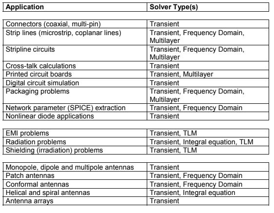
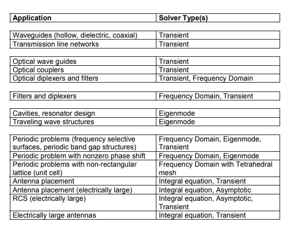
One situation doesn’t always correlate to only one solver, so it is not included in the discussion above about each individual solver. The user must select the appropriate solver himself/herself, but the following section will give some guidelines (NOT RULES) about when to use each solver. IT IS GOOD PRACTICE (according to CST at least) TO RUN BOTH TIME DOMAIN SOLVERS AND FREQUENCY DOMAIN SOLVERS AND COMPARE THEIR RESULTS. This is because the frequency domain solver by default uses tetrahedral mesh, while time domain solvers use hexahedral mesh. In addition, each use different techniques to solve a given problem. By using two entirely independent methods, this allows for consistency checks when comparing the solutions that each solver gets. If both return the same results, then you will have more certainty in the behavior of the structure.
This table is what CST suggests using as the solver with the given application. **THESE ARE GUIDELINES NOT RULES**
Using the Solvers
I will go in depth with the time domain and frequency domain solver, because the others have far more limited applications and these are the most useful. The integral equation solver shares many options with the FDS, so look at that description. I will skip redundant explanations, so if you don’t see one that you are looking for try searching the explanations above it.
1
2
3
4
5
6 7
8 9 10
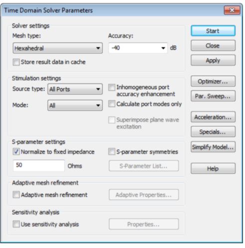
Time Domain Solver Parameters:

12
3
 Algorithm Settings: The parameters that you have set will appear here, and you can change the ranges (using the reset min/max) and use previous results or the current values for each one.
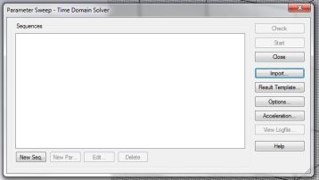 Parameter Sweep: After defining parameters, you can define how you want CST to sweep through them. To do this, click New Seq. and then New Par…, and this brings up another window that is mostly self-explanatory. You can choose if you want the parameter to vary linearly, logarithmically, etc. and then how large you want the steps to be. See sensitivity analysis to learn how to create a parameter.
a
b
c
d
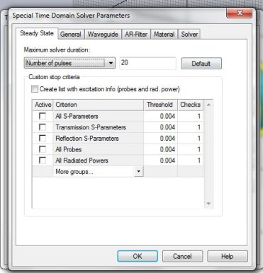 Specials: This has some special settings for each solver. I will go over the important tabs.
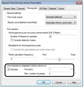 Waveguide: In this tab, one of the most important sections is at the bottom in the box. This is where you can define how accurately you want CST to do mesh refinement. The accuracy value in percent indicates how small you would like the truncation error to be.
Frequency Domain Solver
1
2
FDS: After results are calculated, you can use the axis marker to choose a location and calculate additional fields at the axis marker at points of interest and doesn’t require another simulation run. Data on the fields between steps is stored, so it doesn’t matter which point is chosen.
Brief Description of the Computational Methods of CST Solvers
(At the request of Peter)
Finite Integration Technique:
The basic approach of this method is to apply Maxwell’s Equations in integral form to a grid (i.e. the mesh) of discrete locations. This is an extremely useful method for modeling, because it is memory-efficient and allows for flexibility in using different materials and geometries. The goal when using this technique is to limit the error that occurs due to discretization.
Within each individual meshing, the calculation takes place by applying electric grid voltages across the edges and magnetic fluxes across the faces of the grid.
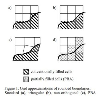 Perfect Boundary Approximation:
The perfect boundary approximation is where CST adjusts the edges of the meshing around boundaries so it can better simulate the behavior around boundaries. This is especially important since the behavior around boundaries varies much more greatly due to the geometry of the device where other locations do not.
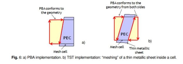
Thin Sheet Technique:
Below is a picture of the Thin Sheet Technique. It is essentially an extension of the PBA. When there is a thin sheet of material that is thinner than the thickness of a mesh cell, the thin sheet technique uses the PBA on both sides of the thin sheet, in order to avoid situations like a) within the diagram. B) is where TST is applied.
Transmission Line Method:
The TLM method is where each meshing is considered as a transmission line, and a way to simulate the propagation of a wave. At a point where an EMW meets another meshing, the wave scatters along the edges of adjoining mesh. Thus, there are three transmitted waves (one in each direction, where in this case we are considering a 2D figure) and one reflected one. Then, these transmitted and reflected waves excite the nearby nodes in those adjoining meshes. For a better description, please see https://en.wikipedia.org/wiki/Transmission-line_matrix_method .
Multi-Level Fast Multipole Method:
This is the same as the Method of Moments, but with less time complexity so that the simulation can run faster. This uses boundaries conditions in order to solve integrals to equations where Green’s functions can be applied